Definitions

With:

• \(M\), a basis matrix containing the basis vectors as columns
• \(\vec{v}\), a column vector in the basis vector space \(M\)

When written as:

the vector \(\hat{a}\) is the vector in global coordinates.

The reverse can be achieved to determine a vector defined by a different basis:

This works both for 2-D and 3-D vectors.

Example

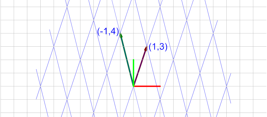
Let a set of basis vectors be defined as:

and

The basis matrix being:

These basis vectors result in the following grid when plotted:

Conversion to Global Coordinates

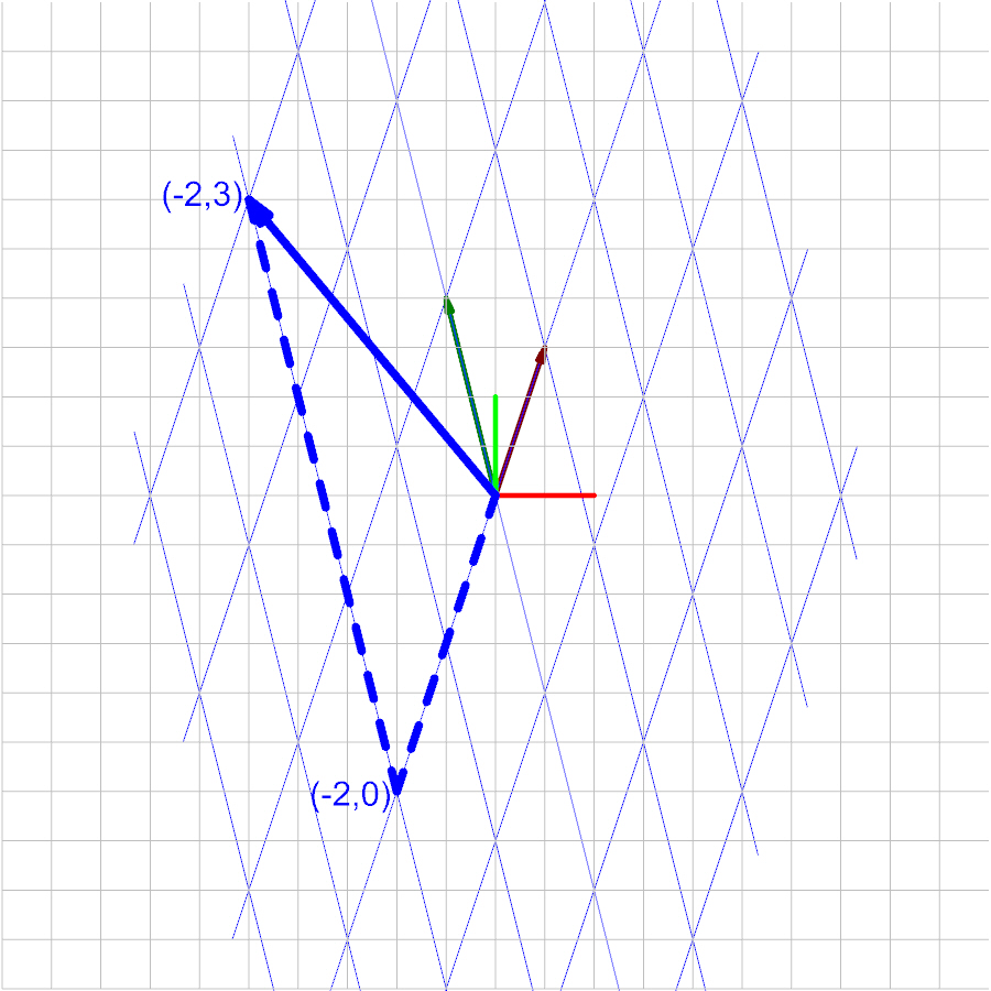
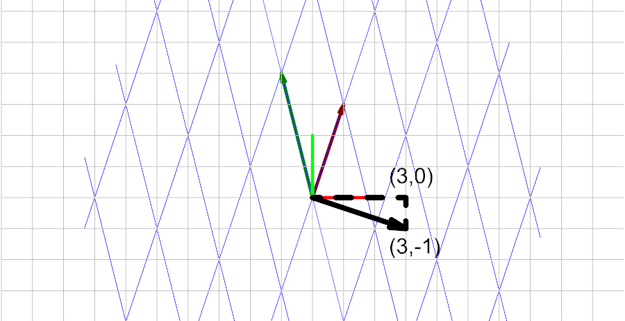
Set a vector in this space  equal to \(\begin{bmatrix}-2&3\end{bmatrix}\).

This vector using basis coordinates is plotted as the following:

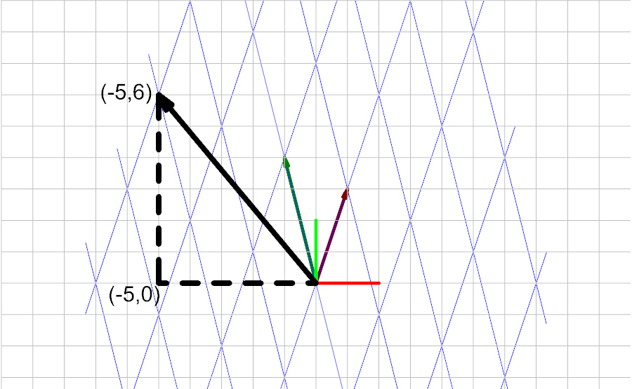
The vector \(\vec{a}\) (in global coordinates) is calculated with Eq 1. and is therefore equal to

Converstion to Basis Coordinates

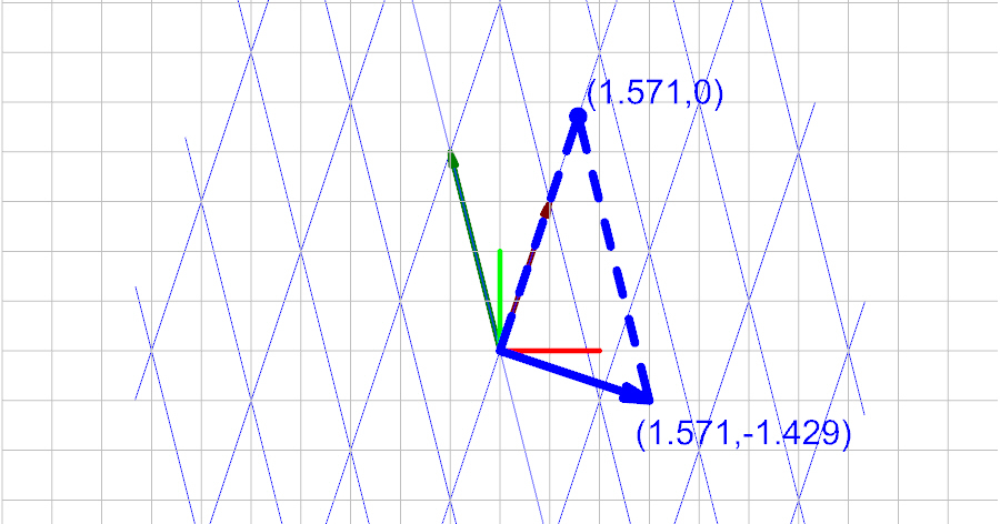
Using a vector in global coordinates of:

we have:

And to convert it to the basis space, we multiply the vector by the inverse of the basis matrix.

Transformation Matrix

Change of basis can be used to derive transformation matices.

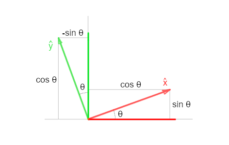
Rotation

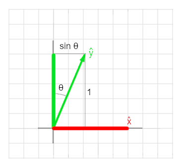
Counter-clockwise rotation by an angle \(\theta\) is developed using unit vectors established by this angle:

\begin{equation*} \hat{x}=\begin{bmatrix}\cos{\theta}&\sin{\theta}\end{bmatrix} \end{equation*}

\begin{equation*} \hat{y}=\begin{bmatrix}-\sin{\theta}&\cos{\theta}\end{bmatrix} \end{equation*}

\begin{equation*} M_{rotate}=\begin{bmatrix}\cos{\theta}&-\sin{\theta}\\\sin{\theta}&\cos{\theta}\end{bmatrix} \end{equation*}

Scale

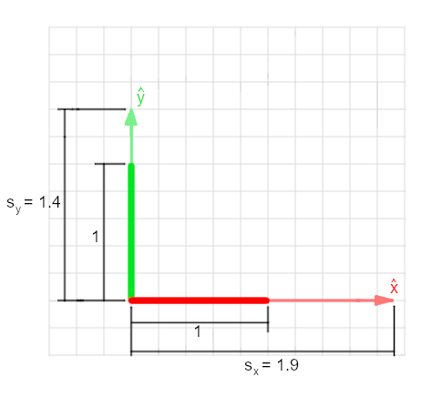
With scaling, the global unit vectors maintain the same orientation but are scaled in length by a scale factor, \(s\). The new basis vectors are then the following:

\begin{equation*} \hat{x}=\begin{bmatrix}s_x&1\end{bmatrix} \end{equation*}

\begin{equation*} \hat{y}=\begin{bmatrix}1&s_y\end{bmatrix} \end{equation*}

\begin{equation*} M_{scale}=\begin{bmatrix}s_x&1\\1&s_y\end{bmatrix} \end{equation*}

Shear

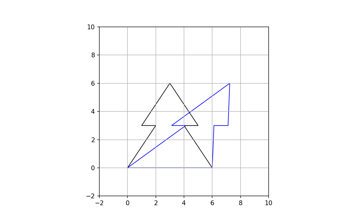
Shearing along a principal axis may be derived as follows, for example when along the x-axis:

\begin{equation*} \hat{x}=\begin{bmatrix}1&0\end{bmatrix} \end{equation*}

\begin{equation*} \hat{y}=\begin{bmatrix}\sin{\theta}&1\end{bmatrix} \end{equation*}

\begin{equation*} M_{shear,x}=\begin{bmatrix}1&\sin{\theta}\\0&1\end{bmatrix} \end{equation*}

Polygon Transformation

As an example of transformation matrices, let's create and transform a generic polygon using Python and matplotlib.

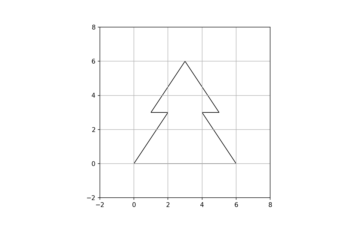
Using the following points as definition:

xy = np.array([[0,0],[2,3],[1,3],[3,6],[5,3],[4,3],[6,0]])

we obtain this polygon:

Rotation

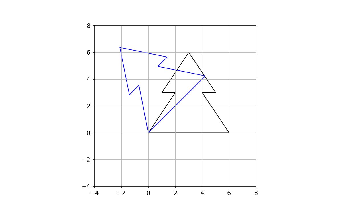
For a rotation of 45 degrees, counter-clockwise about the origin, the transformation matrix becomes:

rotation = np.radians(45)
x = np.array([  np.cos(rotation), np.sin(rotation) ])
y = np.array([ -np.sin(rotation), np.cos(rotation) ])
M = np.hstack( (x.reshape(-1,1), y.reshape(-1,1)) )

>>> print(M)
[[ 0.70710678 -0.70710678]
[ 0.70710678  0.70710678]]

The new polygon points are then calculated with:

xy_new = np.dot(M,xy.T)

Adding the rotated polygon to the plot:

Scale

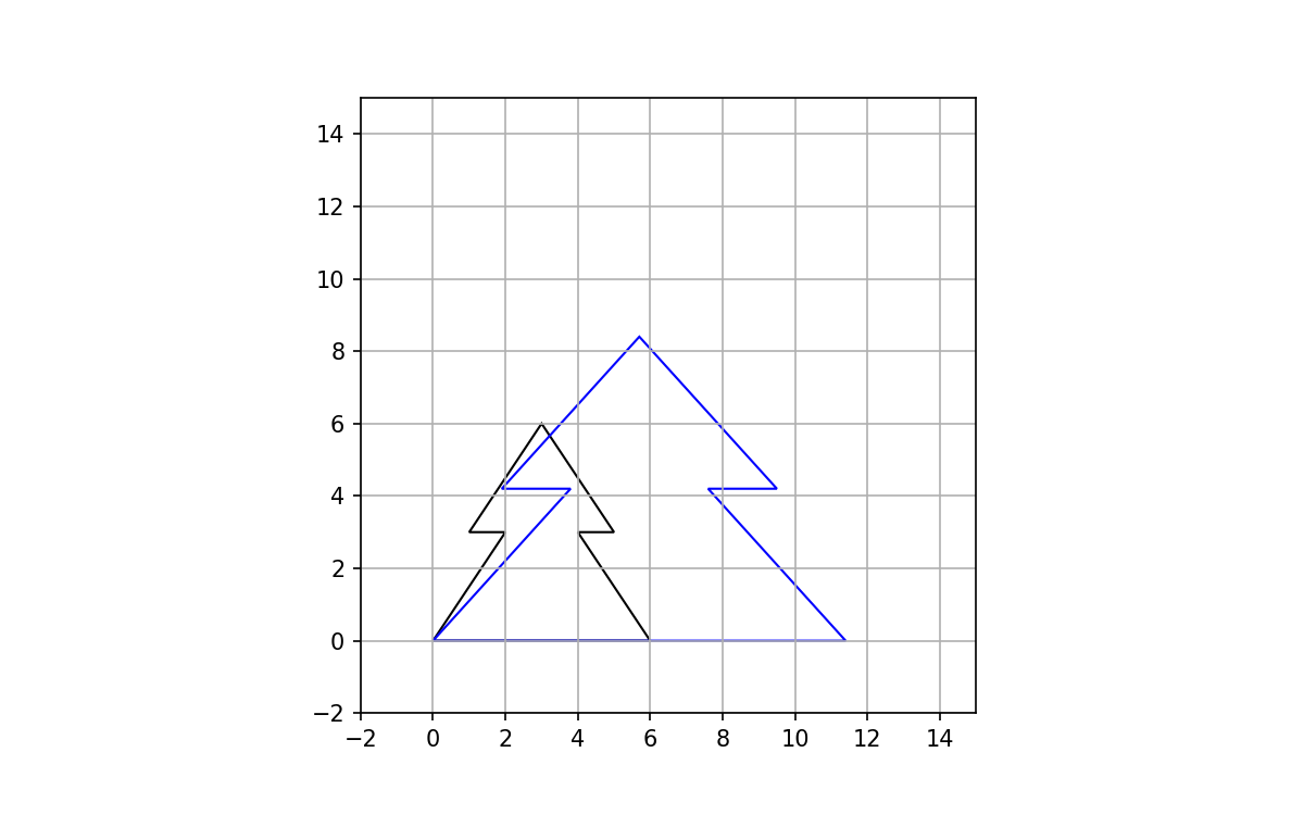
Using scale factors of 1.9 and 1.4 for the x and y axis, respectively:

sx = 1.9
sy = 1.4

x = np.array([ sx, 0 ])
y = np.array([ 0, sy ])

M = np.hstack( (x.reshape(-1,1), y.reshape(-1,1)) )

>>> print(M)
[[1.9 0. ]
[0.  1.4]]

We calculate the points for the scaled polygon the same way:

xy_new = np.dot(M,xy.T)
poly_scaled = Polygon(xy_new.T, fill=False, edgecolor='blue')

And plotting:

Shear

Here we will shear along the x-axis by 45 degrees. The transformation matrix is:

angle = 45

x = np.array([ 1, 0 ])
y = np.array([ np.sin(np.radians(angle)), 1 ])

M = np.hstack( (x.reshape(-1,1), y.reshape(-1,1)) )

>>> print(M)
[[1.         0.70710678]
[0.         1.        ]]

And the sheared polygon is calculated using matrix multiplication again:

xy_new = np.dot(M,xy.T)
poly_scaled = Polygon(xy_new.T, fill=False, edgecolor='blue')